Gaussian guide
Preamble
- This guide will serve to help you do simple DFT calculations with the Gaussian software, a popular tool for quantum chemical calculations, in the NCI Gadi system.
- To first access Gadi, you need to install your preferred remote access tool. MobaXterm is great on Windows and I think it should be installable for Mac. MobaXterm is quite powerful as it can access GUI software like GaussView or VMD from Gadi using Xterm. If you are using Mac you can remotely access using the terminal.
- The next step is to acquire a File Transfer Protocol (FTP) client for downloading and uploading files into or from Gadi. I use WinSCP and for Mac there is Filezilla or Cyberduck. In Mac you can also use the Terminal (similar to Linux environment) to transfer files between your computer and NCI’s Gadi, see tips here.
- The command to transfer to Gadi:
scp yourfile userid@gadi.nci.org.au:/somepath/folder -
From Gadi to your computer:
scp userid@gadi.nci.org.au:/somepath/folder/yourfile - For more information on Gadi and useful basic commands on Linux:
Preparing Gaussian file
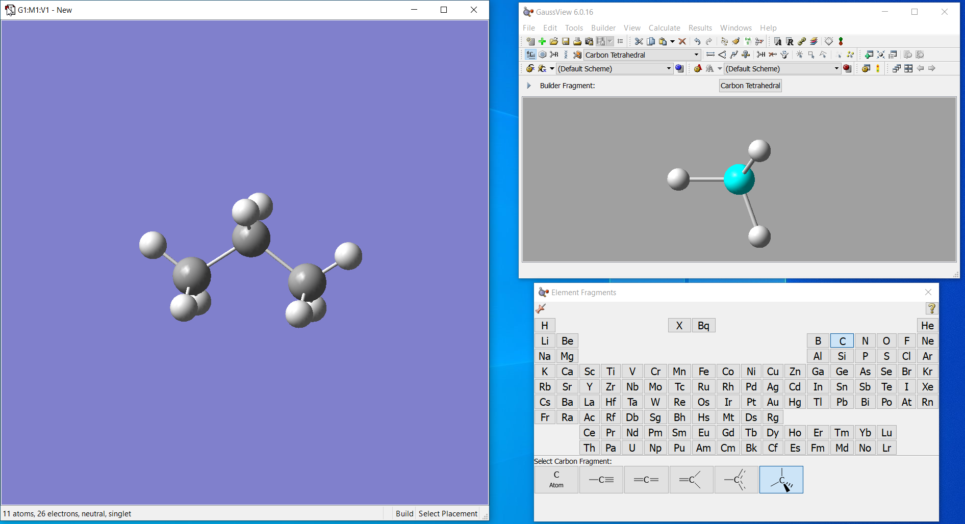
- You can use any molecular GUI available like GaussView (GV), Iqmol, Spartan or even Avogadro to construct your structure. Here I made propane with GV.
-
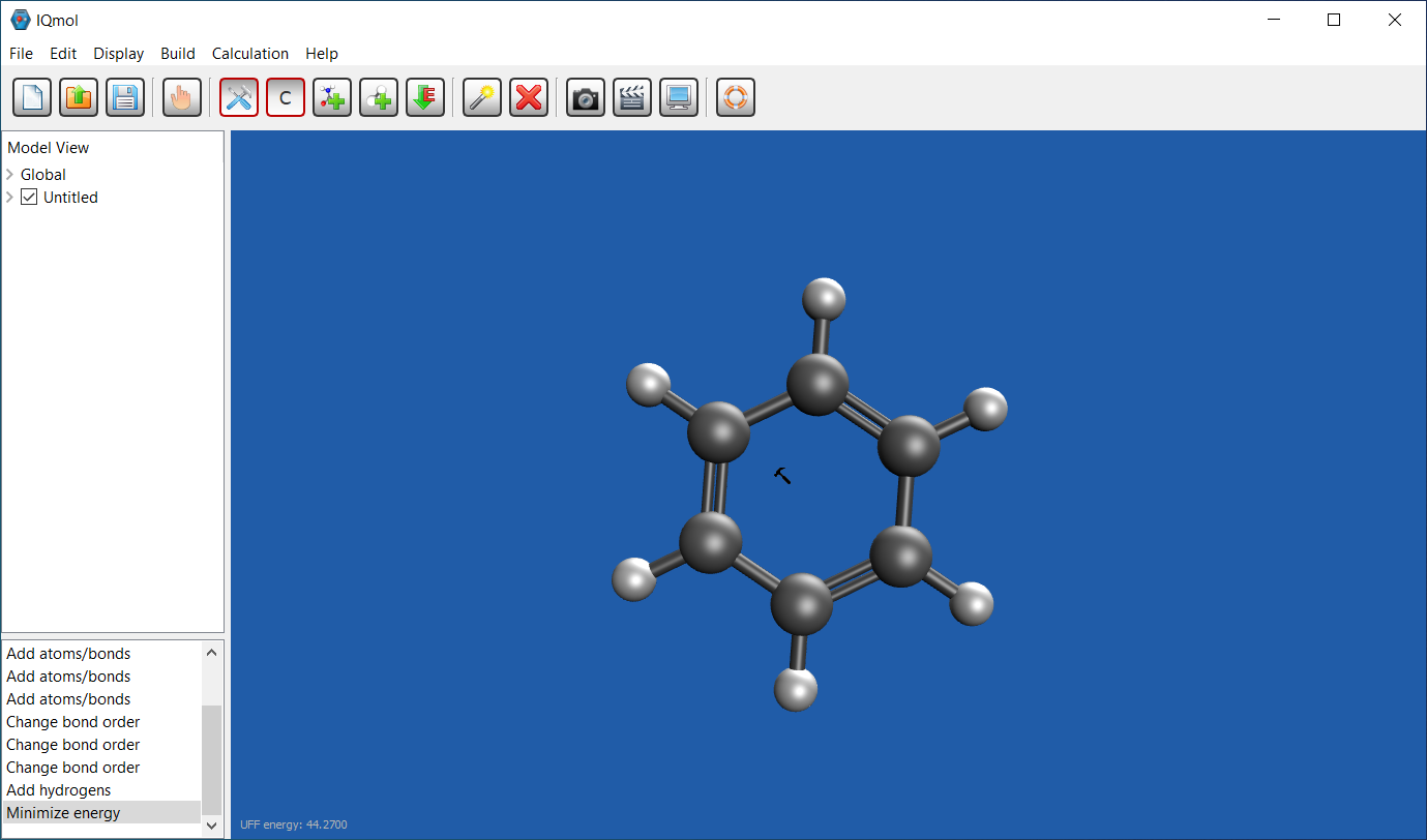
Iqmol (IQ) is a free software and you can download from here. It is available on both Windows or Mac. I made a benzene ring here. It is highly recommended that you read the guide for these programs too.
-
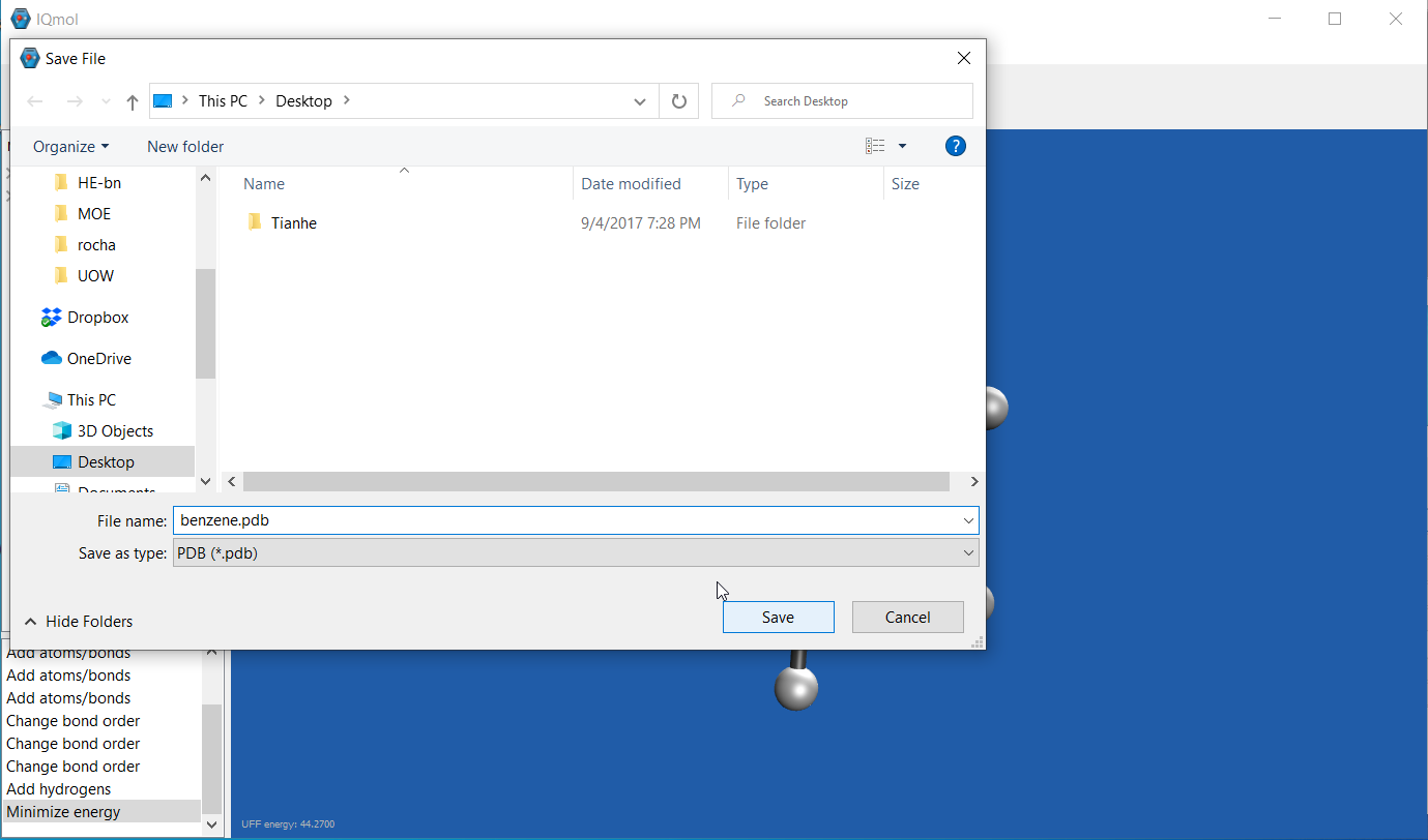
Once done, save the file into format that can be read by GV, i.e. .xyz or .pdb formats if you are using IQ.
-
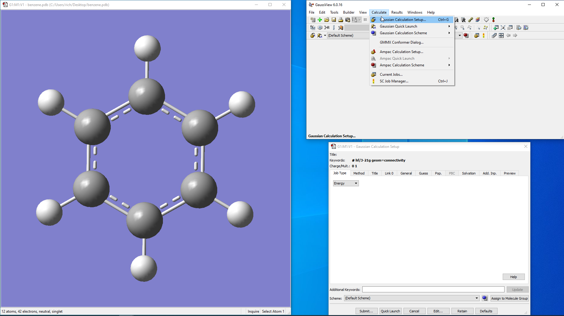
For.pdb files you will need to open using GV, export and save it as the gaussian input file format .gjf. To do a proper conversion from .pdb to .gjf it is a little complicated. To do so, once you’ve loaded bezene.pdb in GV, go to >Calculate>Gaussian Calculation Setup…
-
In the Setup panel click on ‘General’ tab:
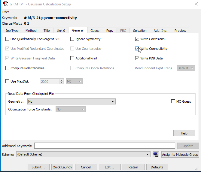
- Untick the ‘Write Connectivity’ and ‘Write PBD Data’ options but keep the ‘Write Cartesians’. Then click on ‘Submit’, and save the file as .gjf. If it prompts you to Submit the job into Gaussian click ‘No’.
Gaussian input
-
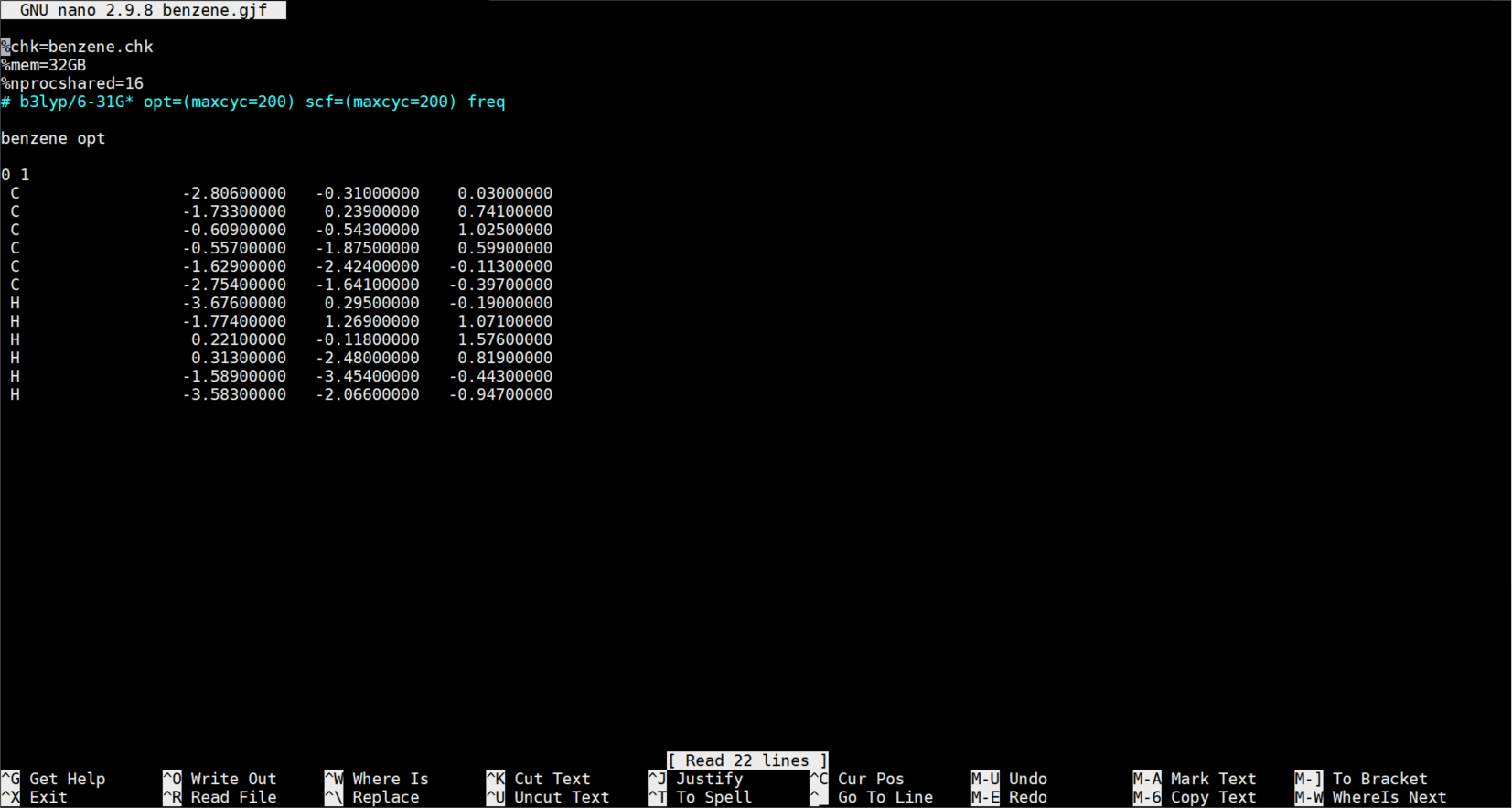
Before sending the job to run in Gadi, you need to edit the benzene.gjf file with Notepad++. This editor is also useful for coding. You can use any editor tools you prefer.
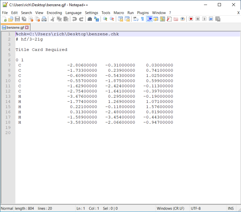
- You can see the xyz cartesian coordinates of the atoms above. Another way of organising the atoms’ 3D information is the z-matrix format which we use to do PES scans.
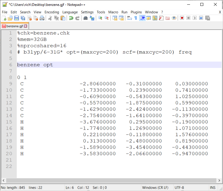
- Here are the edits you need to do on your raw gjf file in notepad++:
- Rename the
%chkto benzene.chk (this is checkpoint file) - Add
%mem=8GB(To request 8GB memory in a node. This is different from the image.) - Add
%nprocshared=4(to request 4 cpus in a node. This is different from the image.) - Add the optimization for minimum structure optimization:
# b3lyp/6-31G* opt=(maxcyc=200) scf=(maxcyc=200) freq- If you are calculating a transition state:
# b3lyp/6-31G* opt=(ts,calcfc,noeigen,maxcyc=200) scf=(maxcyc=200) freq- If you’re doing potential energy surface (PES) the atoms need to be in z-matrix format
- Insert comments or the job title. Important: note the one black space after the keywords and one blank space after
- 0 1 – refers to 0 as the charge (this is a neutral structure) and 1 as the spin multiplicity
- After the xyz leave 2 blank lines - this is important!
- Rename the
Submitting job
- If this is your first time setting up in Gadi, you will need to setup your own folder:
- Change directory (CD) to zl12 project folder:
cd /g/data/zl12/- Make your own directory:
mkdir <user_id>- CD to your directory:
cd <nci_id>- Make your own project folder:
mkdir <project_name>- Your calculations will be placed in this project folder and whenever you run jobs wish to view them jobs you can CD:
cd /g/data/zl12/<user_id>/<project_name>- Note: your project name or files must never have spaces or special chars between them like ‘proj 1’ or ‘proj&1’. You should instead name them as ‘proj_1’ or simply ‘proj1’
-
To edit a new file in the bash you can either use
nanoorvi. Personally, I prefernano:
-
Copy and paste over the lines in benzne.gjf you saved in your editor to MobaXterm (just do a right click). Save and exit by ‘Ctrl-X’.
- Use the script
_g16to run the benzene.gjf job. Or you can simply make one withnano:
#!/bin/bash
## To submit, ./_g16 <filename> <time> <cpu> <mem>
## (with or without .gjf extension; time in hrs otherwise default is 24 hrs;
## cpu default is 4; memory default is 8GB)
## Edited 20/4/2020 ~Richmond
## Input variables:
INPUT=`basename $1 .gjf`
TIME=${2:-24}
CPU=${3:-4}
MEM=${4:-8GB}
JOBST=128GB
PROJ=zl12

## check if job exists
if [ ! -e $INPUT.gjf ]; then
   echo "   -> !!!!! [$INPUT.gjf] does not exist !!!!! "
   exit -1
fi

cat << EOF > $PBS_O_WORKDIR\g16.sh
#!/bin/bash
#PBS -l walltime=$TIME:00:00
#PBS -l ncpus=$CPU
#PBS -l mem=$MEM
#PBS -l jobfs=$JOBST
#PBS -l storage=gdata/zl12
#PBS -l wd
#PBS -e $INPUT.e
#PBS -o $INPUT.o
#PBS -N $INPUT
#PBS -P $PROJ

echo "Started job on `date` "

cd \$PBS_O_WORKDIR

cpulist=`grep Cpus_allowed_list: /proc/self/status | awk '{print $2}'`
echo "%CPU=$cpulist" > \$PBS_JOBFS/\$INPUT.gjf
cat \$INPUT.gjf >> \$PBS_JOBFS/\$INPUT.gjf

module load gaussian/g16a03
g16 -P=$CPU <$INPUT.gjf> $INPUT.log 2>&1

EOF

qsub g16.sh

echo "   -> Job [$INPUT.gjf] submitted! $CPU cpus; $MEM mem; running $TIME hrs"
- It is important to ensure that the
_g16file is executable by doingchmod +x _g16. - You only need to do this once and executable files are green in MobaXterm.
- To run the benzene.gjf job, you need to dispatch the job to a PBS Pro scheduler or normally what we do is to
qsubbut I’ve already added this command into the_g16script so not necessary toqsub. You can look at the script’s code if you’re interested. I’ve set all the parameters to run the job using resources but you can change them as you like for default. - Finally to submit the job type in the directory where your file is:
./_g16 benzene. You’ll need to include the filename and time which I put as default of 24 hours. - The job-hours depend on what kind of jobs you are running. Obviously, PES will usually be longer say 48 hours and you can submit by
./_g16 <file_name> 48(which is the maximum run-time in Gadi). In this example, the benzene calculation takes only a few seconds! Note that the PBS will return a 4213261 which is the job ID. And if successful there will be an echo out of the job status.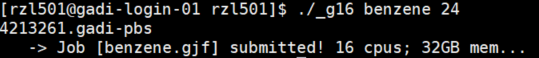
Checking job status
-
You can check all jobs running by
qstat -u <userid>: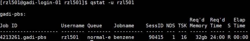
- Or you can directly
qstatthe jobid byqstat -f. - To stop the job you can
qdel <job_id>. -
Once the job is completed, there will be no more lines when you
qstat. When the job is being run, a benzene.log file is being created. If youtail benzene.loga completed log file you will see some quotes and a ‘Normal termination of Gaussian 16 t …’ line: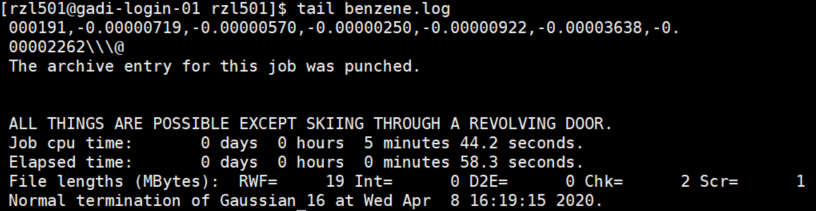
- Transfer this file into your own computer harddisk using the FTP client.
Viewing completed jobs
-
You can view the benzene.log with GV in the MobaXterm by typing
gview benzene.logor alternatively if you have GV installed in your computer you can view it from there. But this is the view of the completed structure. Near the green button you see 3 of 3 which meant that this job took 3 steps to complete because our guess structure is very close to the electronically optimized one at B3LYP level of theory.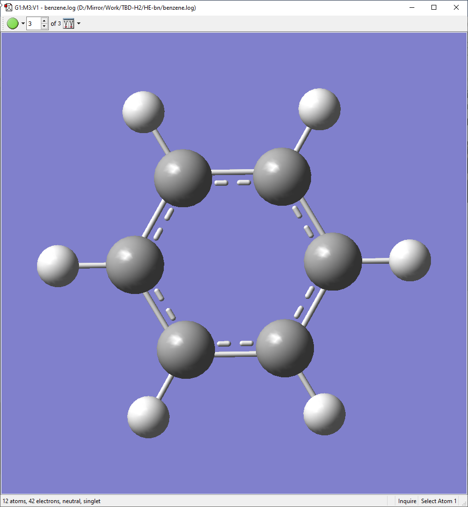
-
Click on the panel with the ‘Results’ tab to see the summary of the calculations.
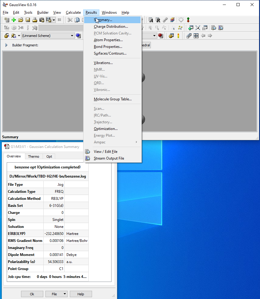
-
Under the ‘Thermo’ tab, there will be some values we are interested in, i.e. the ‘Electronic Energy’, and ‘Thermal correction to Free Energy’.
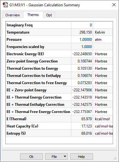
- To find the free energy of this structure, we add the EE + Thermal Free Energy Correction (fourth line from the last). If you’re looking at the enthalpy, then is EE + Thermal Enthalpy Correction. Note that all this are taken at 298.15 K. Since we know that G = H – TS, the entropy is just (H – G)/T.
- More one final important thing to check is that the vibration frequencies (goto >Results>Vibrations…) do not have imaginary values, i.e. all the values are positive for a minimum structure. Transition states have a value which is negative. Usually imaginary frequencies will show up as negative in Mode #1.
Potential energy surface
- Here I will show you the steps in running a PES scan to locate transition state (TS) structure and the corresponding minimum.
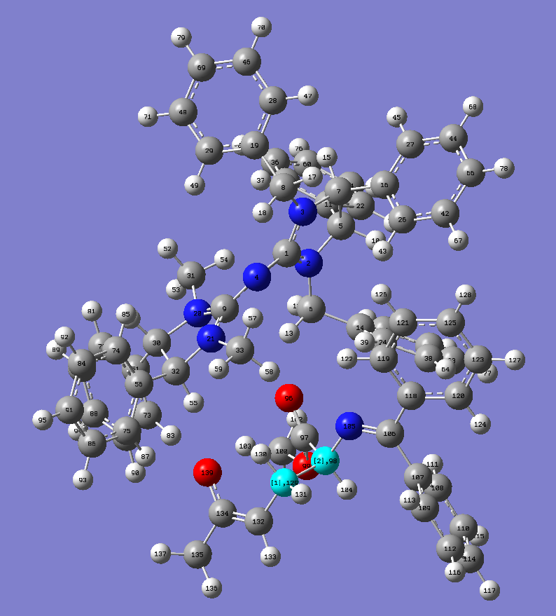
-
First I open a completed or optimized .log file in GV. This is a minimum structure of a Michael addition reaction run previously and I am using the structure after the C-C bond is being formed, ie the Michael adduct. For the structure below we are going extend the two highlighted carbon atoms labelled 98 and 129 (select Label under View):
-
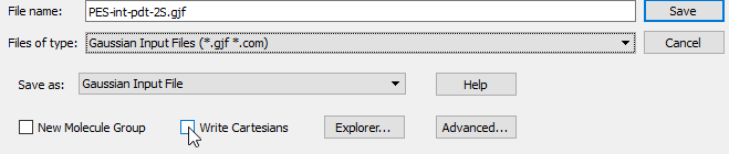
Save the file as ‘PES-xxx.gjf’ and in the save option, remember to uncheck the ‘Write Cartesian’:
-
Load the ‘PES-xxx.gjf’ in notepad++:
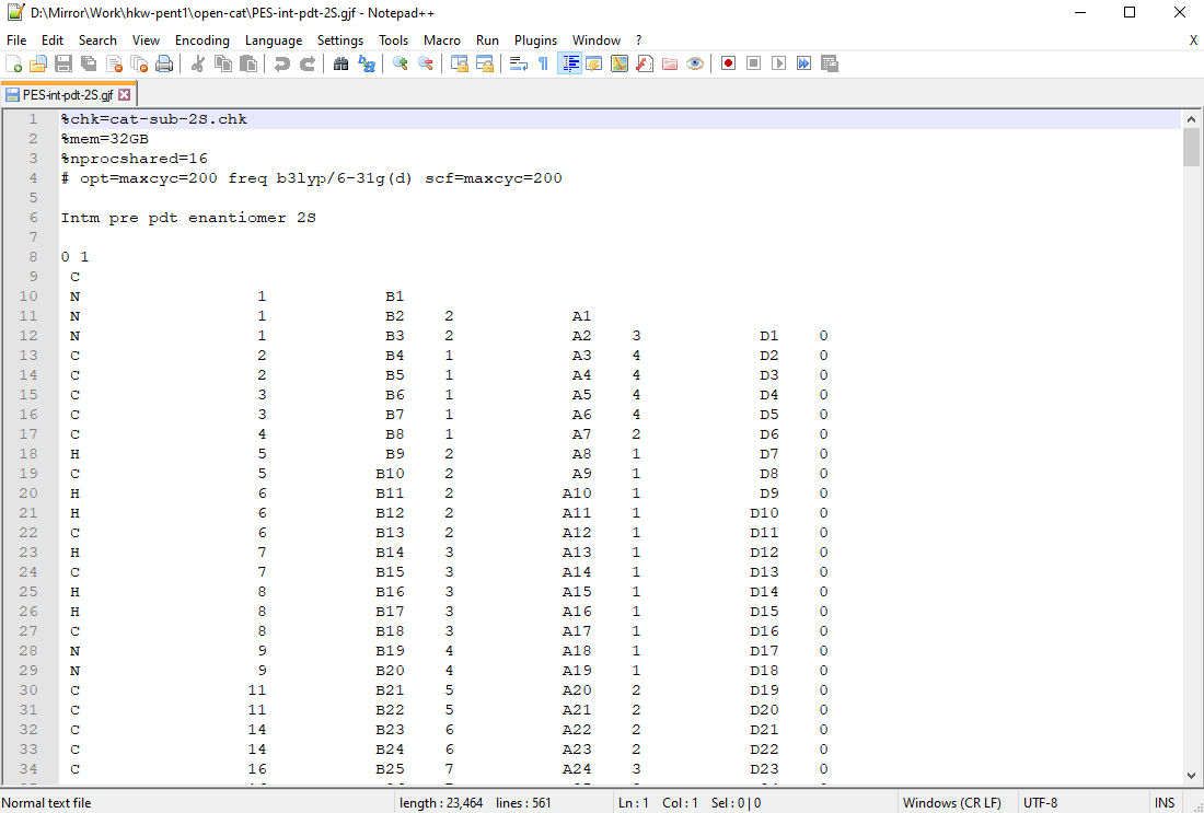
-
You will find that the atom format is quite unlike the one previously used in calculating the benzene minimum structure which was in cartesian or xyz. The format here is z-matrix or z-mat and will be used primarily for PES. To format a PES .gjf file, there are several important edits required in the route as well as after the z-mat:
-
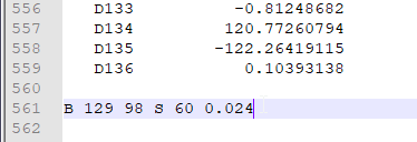
And at the end of the z-mat is the modredundant parameters:
- Here are some of the important key-points:
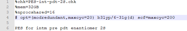
- Check that the name of the
%chkis correct. And there are no spaces or special chars. - Add the option ‘modredundant’ and change to
maxcyc=20in theoptor optimization keyword. There is no need forfreq– it is only required for optimization jobs. - Edit the title to indicate that this is a PES job.
- After the tail end of z-mat add one blank space and key in the desired bond/angle/dihedral to manipulate. In this tutorial, the modredundant command
B 129 98 S 60 0.024translates to a relaxed scan of the bond between atoms 129 and 98, scanning 60 steps and each step the distance to lengthened by 0.024 Å. Conversely,B 129 98 S 60 -0.024would result in the atoms 129 & 98 being brought closer. - How do I determine how many steps to run? This is really based on guestimation, intuition and experience. But usually for TS structure dealing with C-C bond addition, I would expect the distance to be about 2.5 Å based on my experience. As the minimum C-C bond is about 1.4 Å, I would expect after 41 steps, it would have reached 2.5 Å and the TS structure. The step size of 0.024 will usually give us a nice PES profile (see section on PES scan example). However, sometimes I will run step size of even 0.05 to get a rough estimate to cut down on computational time and cost. The con is that the PES profile might not give a clear sign of TS.
- The order of the atoms is important - 129 comes first as I want atom 129 and its connecting group of atoms to translate rather than atom 98 and its connecting group of atoms. You will see this once the job is run.
- Finally, it is very important to leave a blank space or a few bank spaces after the command.
- Check that the name of the
PES for dihedrals and 3D scans
-
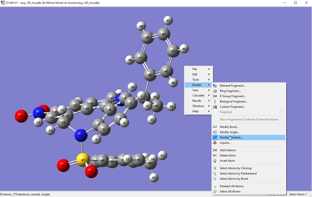
Load the optimized structure in GV, and right click to then go to >Builder>Modify Dihedral:
-
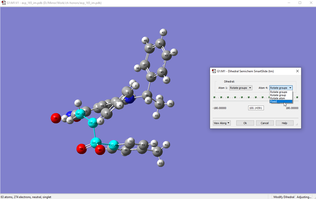
Select atom 49 first, followed by 47, 11 and 12. After that a slider will appear. Fix atom 4 so that only the tosyl group will be rotated:
-
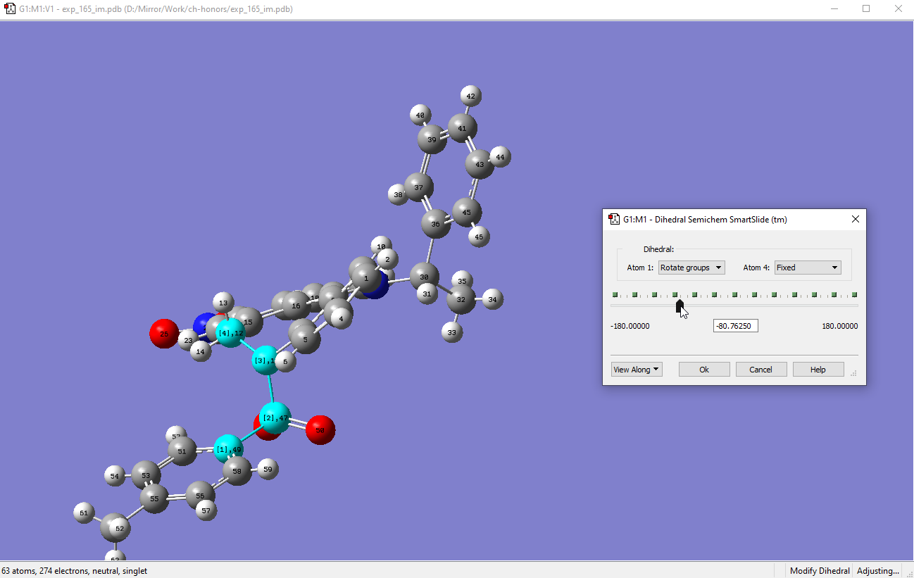
Rotating this dihedral 180o would result in the tosyl group being flipped out:
-
To do the dihedral scan, the modredundant parameters appended at the end of z-mat should be
D 49 47 11 12 S 60 -3.0. This meant by the end of step 60 the dihedral would have changed by 180 degress. Note that the step size decimal .0 is important otherwise there will be an error. -
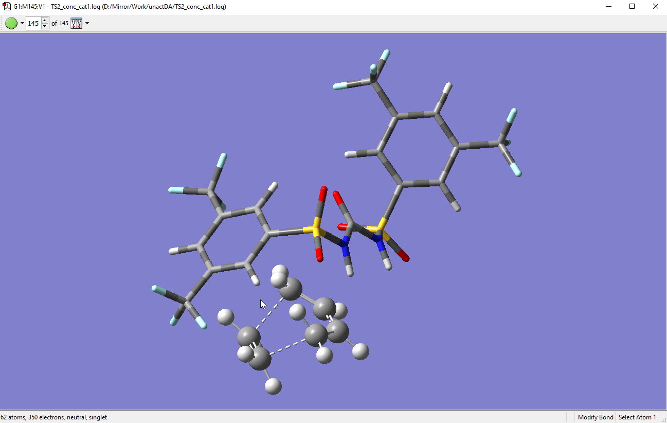
In the case of [4+2] cycloaddition, 3D scans can be performed. However, 3D scans are very slow and long. A strategy to calculate [4+2] is to manipulate the bond distances between the C atoms and run the guess structure as TS. Here is an example of TS for Diel-Alders reaction I calculated. The bond distances between the C atoms (dotted lines) below are an average of about 2.3 Å.
-
To do the 3D scan, the modredundant appended at the end of z-mat should be:
z-mat
<blank>
B ATOM1 ATOM2 S 8 0.1
B ATOM3 ATOM4 S 8 0.1
<blank>
Note that the number of scans here are 8 for each coordinate scan. In fact, there will be a total of 9*9 or 81 steps! That is why the corresponding step size is large, i.e. 0.1 Å. Larger step sizes tend to give very ugly PES profiles, but it can give you a guess structure of the [4+2] structure from which you can optimize. Finally, it is recommended to reduce the size of the structure and use a small basis set, example B3LYP/6-31G(d), to do the scan.
PES scan examples
-
To give you an example, I ran a 3D PES scan PES4-2.gjf for [4+2] between a simple ethylene and diene:
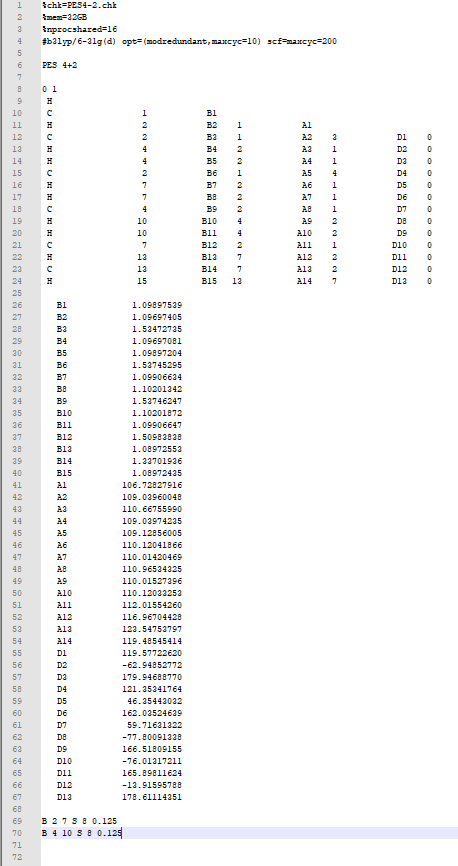
- I decided that a step size of 0.125 and 8 steps for each coordinate should suffice. I am using a commonly used functional or theory which is B3LYP/6-31G(d) or B3LYP/6-31G*.
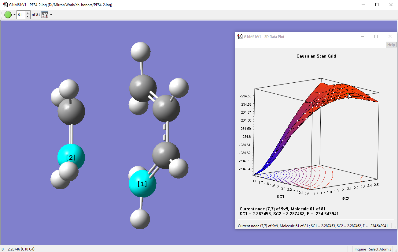
-
After running the scan, below is what I got. As you can see the Data Plot gave a nice 3D plot. What is interesting is that the TS structure sits on a saddle-point:
-
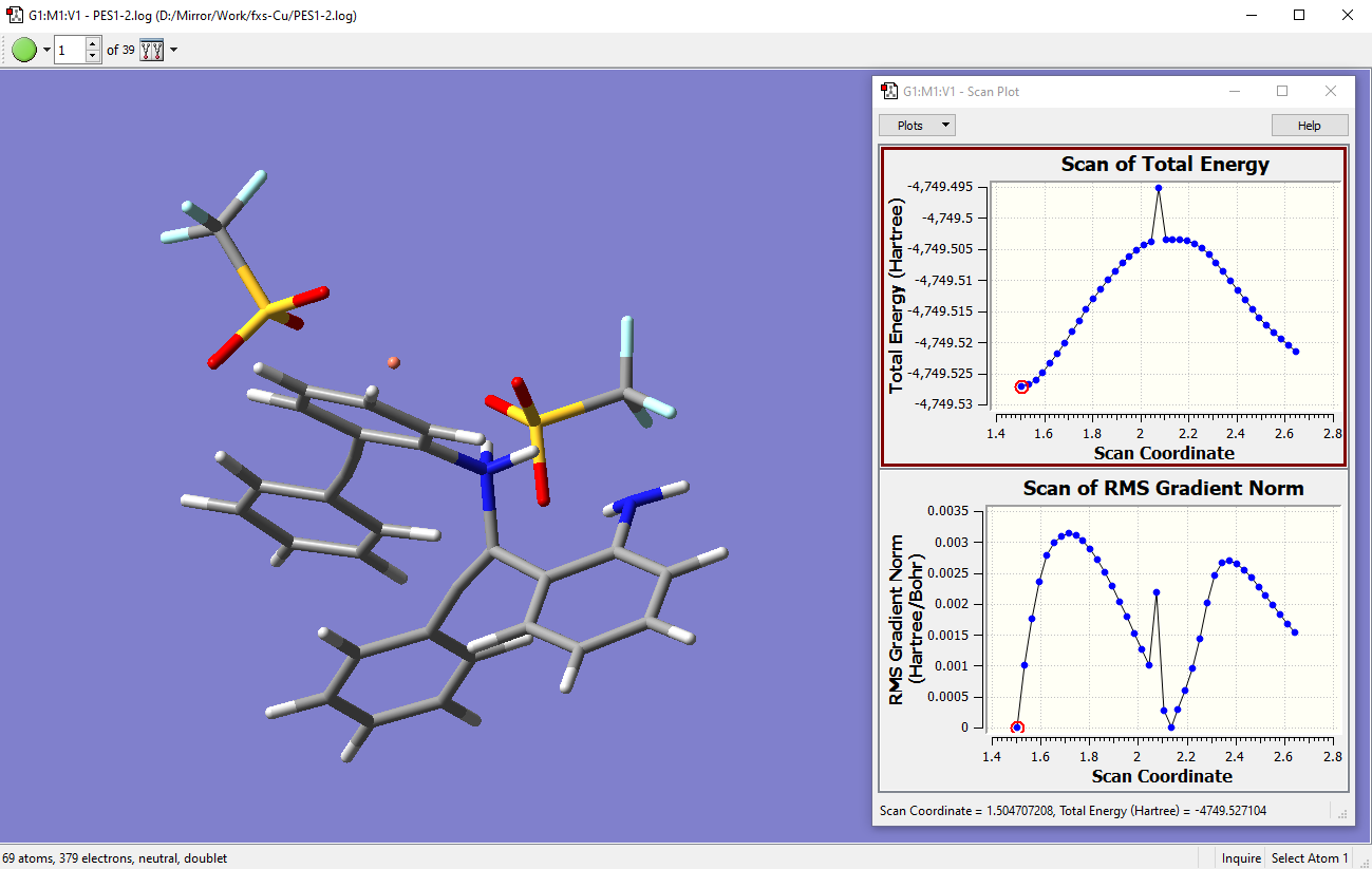
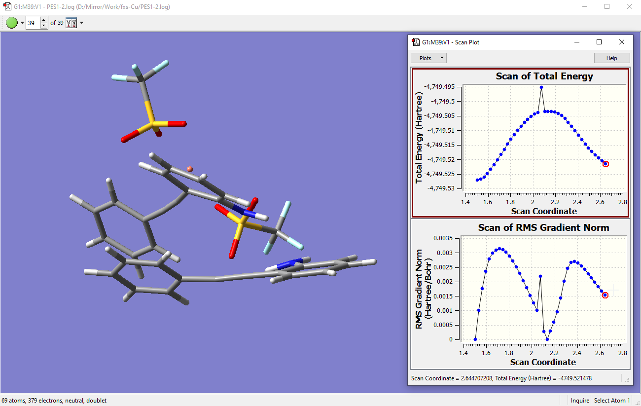
Another example of a PES scan for Cu-catalyzed N-C bond cleavage I calculated. This is the kind of routine 2D PES scan commonly done for most calculations. After doing PES scan calculations, opening the .log file in GV and clicking Results>Scan… will pop up the Scan Plot which is a useful tool for us to visualize the energy surface. A typical ‘ideal’ PES should connect two minimum structures and the top of that ‘energy hill’ should be the TS. The first structure in step 1 of the scan is the minimum optimized earlier:
-
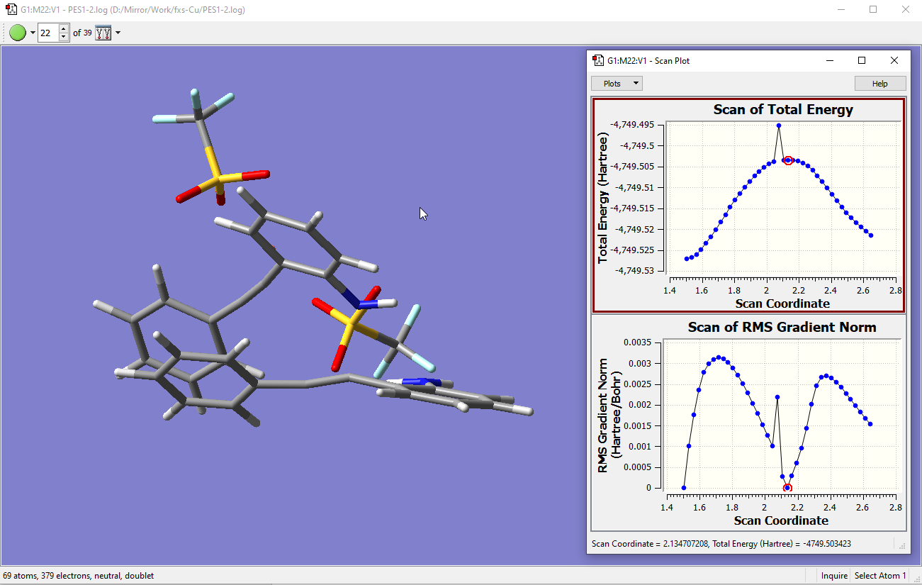
At step 22 shown below is the top of the ‘energy hill’. But depending on the no. of steps in the scan, sometimes the hill can be non-ideal - it is good to still run the TS anyway. Correspondingly the gradient of TS at the top of hill should be close to zero (see below). This is also true for the minimum structure I started with which the gradient is close to zero.
- At step 39, the gradient is converging back towards zero and I would definitely want to optimize that structure as a corresponding minimum which connects from the TS (see below):
TS structures
-
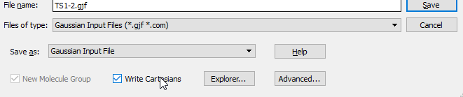
Now to run the TS, simply click on the PES scan plot and select your structure to save. Select the one with gradient closest to ‘zero’. For TS like minimum structures we are using the xyz or cartesian format, so do remember that ‘Write Cartesian’ should be checked:
- Next, open the .gjf in editor and change the keyword route to:
# m11/def2svp opt=(ts,calcfc,noeigen,maxcyc=200) scf=maxcyc=200 freq -
Note that here I am using m11/def2svp as my functional/theory for the calculation here. For starters, you should stick to B3LYP/6-31G(d) as in the previous examples. Note that the
%memandnprocsharedshould be 8GB and 4 respectively for normal Gadi runs: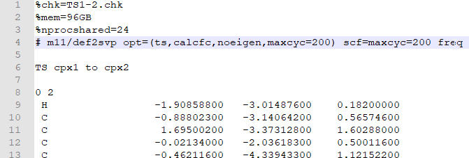
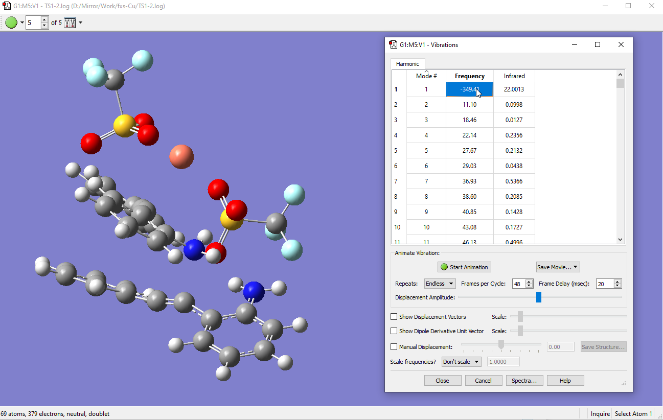
- Once the .log has terminated normally, make sure that you have an optimized TS. Check under >Results>Vibrations and there is only one imaginary (negative) frequency appearing at Mode #1. Here the imaginary vibration is truly a N-C bond cleavage by visual inspection.
Version or changes
First vers. published 30 Sep 2020 Richmond